Neural Networks and how they work

Neural Networks - Explained Easily

What exactly is a Neural Network?

Put simply, a Neural Network, or an NN for short, is a collection of inter-connected neurons that seeks to replicate the way humans think. As such, it is well suited for tasks such as Pattern Recognition and Natural Language Processing that are typically performed by humans.

A Neural Network typically contains Input, Hidden and Output Layers, with connections existing between the neurons in each layer.

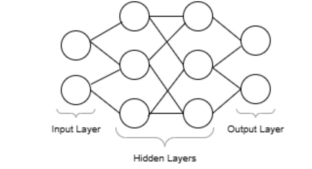
The example above shows hidden layers that are fully connected ( each neuron in the first hidden layer is connected to each neuron in the second hidden layer ), but this is not always the case.

Types of Neural Networks

There are several types of Neural Networks, each serving its own unique purpose. Each type is listed as follows, along with some of its basic, real world applications.

Type of Neural Network	How it's different	Use Cases
Feedforward	Data flows in only one direction - from the input to the output layer without any feedback loops between layers	Pattern Recognition
Convolutional	Leverages convolutional layers to detect information about spatial features such as edges, textures and contours	Image Classification, Object Detection
Recurrent (RNN)	Each neuron's output depends not only on the current input, but also on previous inputs, making RNNs more suitable for sequential tasks	Time Series Forecasting, Language Modeling
Long-Short Term Memory (LSTM)	An RNN that uses a cell states and gates to capture long-term dependencies and overcome the "Vanishing gradient problem" (Discussed later in more detail)	Speech Recognition, Text Generation
General Adversarial Network (GAN)	The Generator and Discriminator (Discussed later in more detail) compete to create progressively more realistic and harder to distinguish synthesized outputs	Deepfakes, Image and Video Generation/ Synthesis
Autoencoder	Uses a combination of an Encoder and Decoder (Discussed later in more detail) to learn the best way to represent input data in a lower-dimensional space	Dimensionality Reduction, Anomaly Detection, Image Compression

The Math behind a Neuron

You now know that Neural Networks are made up of layers of neurons, with each neuron representing a unique node in the network. But did you know that each of these nodes is made up of two parts - a linear equation and an activation function?

Linear Equation

The linear equation defines the relationship between the target variable y and the features xi in the dataset.

$y = w_1x_1 + w_2x_2 + b$

This is done after taking into account the weights w_i associated with each feature, and the overall bias term of the equation b. In the above example, our equation has two features x₁ and x₂ with corresponding weights of w₁ and w₂ respectively. These weights determine the influence of each feature on the overall output.

Similarly, the bias term b allows the model to adjust the output independently of the input values. Finally, the output of this linear equation is passed into an activation function.

Activation Function

As we discussed earlier, each neuron is assigned an activation function. This activation function, when passed the neuron's unique linear equation, determines whether or not the neuron will be "activated" during the current forward pass (we will discuss this later).

Only neurons that have been activated are able to propagate information forward to subsequent layers in the Neural Network. This is known as sparse activation.

Ensuring that only certain neurons are activated during a forward pass can also reduce the complexity of the model and improve its ability to produce accurate outputs for new, unseen inputs. We refer to this as the model's ability to generalize.

Choosing an Activation Function

When selecting an activation function, we must think carefully about the criteria we want to use to activate neurons, as this can influence the way our model learns in the long run.

Some commonly used activation functions are listed as follows, along with when it might be a good idea to use them.

Activation Function	Equation	Use Case
Sigmoid	$f(x) = \frac{1}{1 + e^{-x}}$	Good for binary classification tasks, as the sigmoid function converts inputs to a range from 0 to 1
Rectified Linear Units (Relu)	$f(x) = max(0, x)$	Commonly used  in Deep NN hidden layers - due to the sparsity of neuron activation and overall efficiency
Softmax	$f(x_i) = \frac{e^{x_i}}{\sum_j e^{x_j}}$	Preferred for multiclass classification problems due to its probabalistic output
Leaky Relu	$f(x) = \begin{cases} x & \text{if } x > 0 \\ \alpha x & \text{if } x \leq 0 \end{cases}$	Improves the gradient flow for standard Relu by allowing small gradients for negative inputs
Hyperbolic Tangent (Tanh)	$f(x) = \frac{e^x - e^{-x}}{e^x + e^{-x}}$	Used in hidden layers when you benefit from symmetric neuron activations

We will cover these activation functions in more detail in a later blog, but for now, let's discuss how information is propagated through a Neural Network.

The Forward Pass

The forward pass in a Neural Network is the process by which information moves from the input layer to subsequent hidden layers, and finally, the output layer.

Each forward pass produces an output (or prediction) using the current value of feature weights for the activated neurons. Based on the correctness of this output, weights are updated with each pass, and these updated weights are used to generate a new output.

This is an iterative process that only stops when one of two conditions is met.

1. The accuracy of the output falls within a predefined error threshold,

2. The defined number of epochs is reached

Usually this means our model is fully trained and ready for use! But let's take a closer look at how weights are actually updated at the end of each forward pass, and what this means for the Neural Network as a whole.

Backpropagation

Backpropagation is an algorithm used to update feature weights iteratively while a Neural Network is being trained. It tries to update weights in a way that minimizes the error between the Neural Network's output and the actual output value - also known as the ground truth.

This error can be computed in several ways - from using Mean Squared Error to using Cross Entropy, but we will discuss that in a later blog.

Summary

Great! You just learned how neural networks work! Now let's sum things with a practical example that'll jog your memory.

The problem

Let's say we're using our Neural Network to make a prediction - maybe we want to predict the price of a house. We know that the price of a house can be influenced by several things - it's age, location, square footage, and the number of stories it has. These are our features x_i, each having a corresponding weight w_i. This weight represents how much each feature influences the price of the house. Perhaps the square footage of a house can drive up its value much farther than its age or maybe, the opposite is true.

To learn to predict the price of a house accurately, our model will need to see several examples of houses - what they cost, and how this price relates to the values of their respective features. These are our inputs - the same ones that enter through the Neural Network's input layer. These will look something like the following:

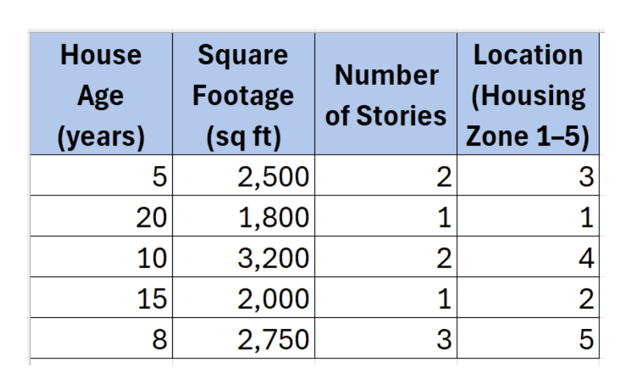
These input features are forwarded into the hidden layers of the Neural Network. There, each neuron assigns different weights and biases to the features in the input to come up with a linear equation unique to that neuron. This linear equation is then passed through an activation function to determine whether or not that neuron will be activated, introducing non-linearity to capture complex patterns.

Activated neurons continue to pass information along the network, until it reaches the output layer, at which point, the model makes its own prediction - the price of the house in question. Remember, the model is still training, and therefore has access to the real value of this house.

After comparing its prediction to the actual price of the house, the ground truth, the model learns how much error exists in its predictions. This information is then backpropagated through the network to iteratively update feature weights for the neurons in each hidden layer.

This process of making predictions and updating weights based on the error in these predictions is iterative, and continues until a good stopping point is reached.

Based on the accuracy of the input data, once its training is complete, the model can predict the price of a house given its features within a reasonable degree of accuracy - even if it has not encountered that specific house in an example before!

So there you have it! That's just one example of the amazing capabilities of Neural Networks. Moving forward, we'll discuss other topics that tie directly into this one, such as Gradient Descent, Prediction, and Classification.